A study of hybrid and chaotic long-range propagation in a double sound channel environment
Abstract : This paper presents the results of the analysis of long range propagation (~200 km) in a range dependent environment. The propagation medium is characterized by two deep sound channels. The range dependence enables energy transfer between the channels and leads to a mismatch between real data and ray predictions. To explain this mismatch, an analysis of hybrid ray propagation is presented. This analysis is completed by an interpretation in terms of chaos. This chaos is quantified in the particular case of the Bay of Biscay environment. This paper puts forward that mesoscale perturbations, such as the Mediterranean outflow in the North Atlantic, can affect long range propagation. However, it shows that the ray theory remains reliable for a propagation range of several hundreds kilometers.
I.
Introduction
The use of Ocean Acoustic Tomography [1] to study large scale oceanographic processes requires that long range acoustic propagation could be efficiently modeled, or, at least, that a good background sound speed field can be found. In this case, usual linear inversion schemes can be applied to estimate temperature and salinity perturbations around the reference ocean. In this context, the presence of sound speed perturbations, which can drastically affect the structure of the sound channel, is a major problem. Indeed, such perturbations can create deep and shallow sound channels, leading to energy coupling and sometimes unpredictability of arrivals at mid and long ranges.
The particular case of the Bay of Biscay, in the North-East Atlantic, is addressed in this paper (Figure 1 ). This region is characterized by the presence of Mediterranean waters outflows. These waters are warmer and denser that surrounding pure Atlantic waters and they stabilized at a depth of approximately 1000 meters. The Mediterranean water outflows create a deep maximum in the sound speed field, leading to the presence of two sound channels in a region of several hundreds kilometers-squared [2]. In 1990, a mesoscale tomography experiment was conducted by the Hydrographic and Oceanographic Office of the French Navy (SHOM). The objective of the so-called GASTOM90 experiment was to test the concept of ocean tomography in an environment where usual linear inversion schemes were suspected to fail [3]. In particular, a major issue of the data exploitation was the analysis of the acoustic propagation and the predictability of ray arrivals for ranges up to 300 kilometers. As presented in [4], a part of the acoustic signals were not predicted by range-independent and range-dependent ray theory. To interpret this mismatch, several theoretical studies, reported in [5], were carried out to describe the behavior and the main features (arrival times and angles) of eigenrays in a stochastic environment. This paper treats the problem of the prediction of the impulse response of the medium, the underlying idea being to explain by simulations the presence of the unpredicted energy in real data. Indeed, the aim of this study is to have a better understanding and interpretation of the propagation in this part of the Atlantic Ocean, in particular in the framework of hybrid ray identification for mid and long range tomography purposes.
This paper is organized as follows: The first section describes the background environment in the Bay of Biscay and presents real data collected during the GASTOM90 experiment. The second section describes a numerical study of propagation in the GASTOM environment, considered as a random sound speed environment. The third section presents a quantification of the chaos degree in the propagation in this realistic GASTOM environment. The aim is, first, to estimate how far a ray model, which is particularly useful to model impulse response because of its small computing time, is reliable in the particular North-East Atlantic environment. Second, the aim is to link the random features observed in real data, as anticipated in [11] with those observed in numerical rays simulations. In the last section, conclusions and perspectives are drawn.
II.
Background environment and example of real data in the Bay of Biscay
A. Background environment
The Bay of Biscay is characterized by the presence of Mediterranean Waters (hereafter MW) issued from the strait of Gibraltar [6]. These waters, constituted by oscillating layers and tongues, are progressively spreading towards the Bay of Biscay and the northern Atlantic. As MW’s are denser than surrounding Atlantic waters, they stabilize around a depth of 1000 meters. They have a high salinity and induce a deep maximum in the sound speed profile. Therefore, the acoustic propagation is governed by a double SOFAR channel environment. A typical sound speed profile is shown in Figure 2. The upper channel is limited upward by the surface (late fall, winter and early spring conditions) or by the seasonal thermocline (late spring, summer and early fall conditions). It is limited downward by the upper Mediterranean waters (roughly down to 1000 meters). The main channel is down limited by the deep layer (~ 3500 meters).
Hereafter, rays propagated in the upper channel are denoted RR+, rays propagated in the main channel are denoted RR- if they are refracted in the seasonal thermocline, and SR if they are reflected on the surface. Finally, rays bouncing on the surface and bottom are denoted SB.
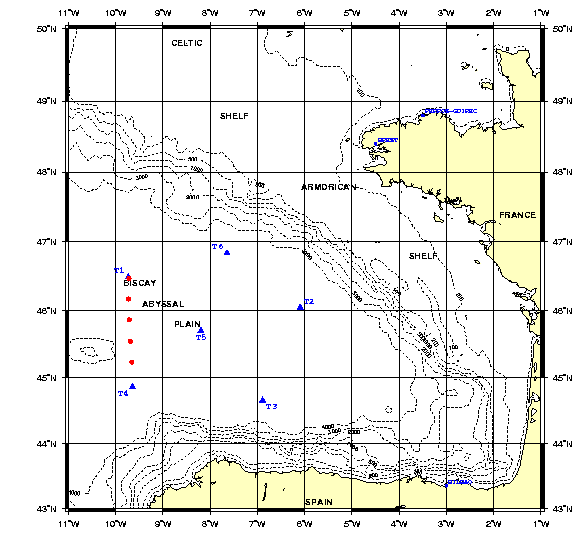
Figure 1: Location of transceivers for the GASTOM tomography experiment. Circles denotes the location of CTD casts between T1 and T4 .
B. Analysis of data
Data presented in this paper were collected during the GASTOM experiment, which was conducted on the abyssal plain of the Bay of Biscay from May to October 1990. Six transceivers were moored at 400 meters to infer the sound speed field between 10°W and 5°W and between 44.5°N and 47°N. The network was pentagonal (Figure 1 ). Propagation ranges extend from 134 kilometers to 307 kilometers. Broad-band signals were periodically emitted (carrier frequency of 400 Hz, bandwidth of 100 Hz). At the receivers, signals were averaged, demodulated, and cross-correlated with a replica of the emitted signal (matched filtering). Transmissions were repeated every 2 hours at the maximum. The acoustic experiment was coupled with several phases of hydrologic surveys including XBT, CTD and current measurements. Additional shallow and deep XBT surveys were conducted along the experiment with particular legs between the locations of the transceivers. In this study, we focus on the T1-T4 leg, which is located on a south-north line. The propagation range is 182 kilometers. The sound speed field, due to the variability in the MW outflow, is range dependent, as shown in Figure 3. This leg is therefore adapted to the study of hybrid ray propagation since the variability of the deep maximum of the sound speed enable energy coupling between the upper and the main channel.
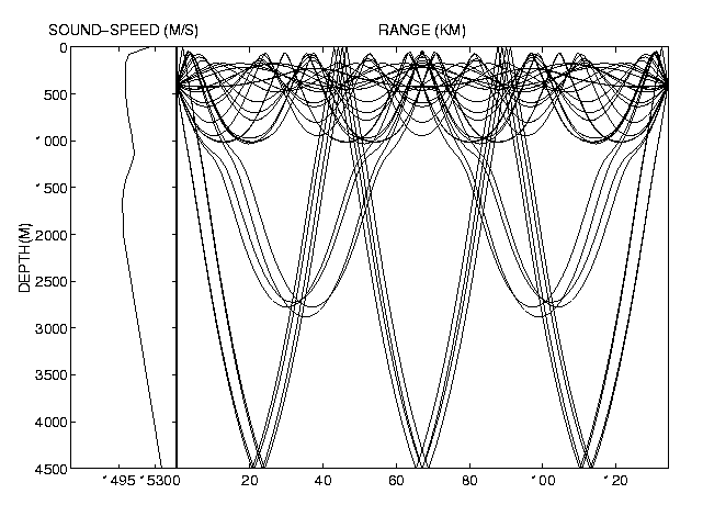
Figure 2: Typical sound speed profile and ray tracing between T1 and T4. The deep maximum in the sound speed profile is due to Mediterranean waters intrusions.
It is shown in [4] that the collected signals are divided into two parts: the first one, with the fastest arrival time, corresponds to the propagation in the upper channel (RR+). It can be noticed that all rays are interfering at the receiver, leading to unresolved arrivals. A second part corresponds to deep refracted rays and/or bottom reflected rays (RR-, SR and SB). Between these two packets, there is some energy which is highly fluctuating but which gets really stable when the signals are averaged over at least 2 days.
Figure 4a gives the averaged real signal collected at T4, exhibiting the two main energy packets and some significant energy with intermediate arrival times (between 121.4 s and 121.5 s). Figure 4b shows the predicted impulse response in a range independent medium obtained by the mean CTD profile; there is a gap between 121.4 s and 121.5 s where no ray is predicted by the range independent theory. This picture represents the impulse response of the sound channel and cannot be directly compared to Figure 4a, which presents the received signal after matched filtering. However, the width of autocorrelation function of the emitted signal is only 20 ms, so that the convolution of the impulse response with the emitted signal cannot spread energy enough to fill the temporal gap and explain the difference of global temporal spreading between measurements and simulations. Figure 4c shows the impulse response of the sound channel in the one realization of a range dependent medium due to the fluctuations of the Mediterranean outflow ; Similarly to the range independent case, no arrivals occur in the gap. Figure 4d shows the impulse response of the sound channel in the another realization of a range dependent medium. In this latter case, some arrival times occur between 121.4 s and 121.5 s ; such arrivals correspond to hybrid rays (trapped alternatively in the upper and the deep channel). They may contribute to the energy packet we would like to explain. The results of figure 4 suggest on one hand that fluctuations of hybrid rays due to random environmental features could explain the energy between RR+ and RR- rays and on the other hand that only a random approach can be reliable. This is the topic of the next section.
III.
Numerical study of the impulse response
The purpose of this part is to identify the unpredicted energy by means of numerical simulations in range dependent environments. The underlying hypothesis is that this energy could come from coupling between the upper and deep channel. The first step is to run a range dependent ray code with a particular environment obtained by a CTD survey between T1 and T4 (Figure 3). The results have shown that at least a part of the intermediate energy packet could be predicted but that the temporal spreading of the first part was not in accordance with data and, moreover, that small fluctuations around the background medium could remove the energy packet or at least change its structure. This suggests that the energy transfer between the upper and the deep channel may be due to small scales fluctuations of the MW. To check this hypothesis, we consider the range dependent medium presented in Figure 3. We superimpose to this medium small scale random fluctuations. Then we compute the impulse response in several environment realizations, and average results over ensemble in order to obtain the mean impulse response.
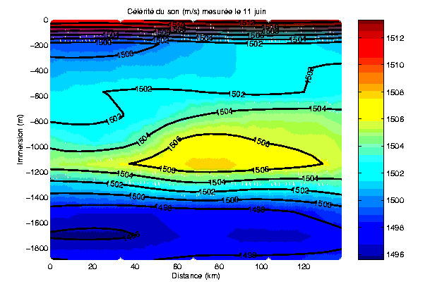
Figure 3: Range dependent sound speed field between T1 and T4. Note the presence and variability of the Mediterranean outflow.
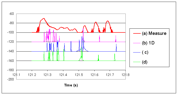
Figure 4: (a) . Averaged signal collected during the period June, 10th – 13th for T1-T4. (b). Predicted impulse response for a range independent medium (bottom reflected rays are the two last arrivals and can be mispredicted due to uncertainty on the bathymetry and bottom nature) (c), (d). Predicted impulse response for two different realizations of a range dependent medium.
A. Model of random fluctuations
We consider the sound speed field as:
C(r, z) = Co(r, z) + dC(r, z), (1)
where Co(r, z) is given by a CTD leg (five profiles) along T1-T4 and dC(r, z) represents the random fluctuations. The fluctuation spectrum is computed from the analysis of all CTD casts done during the GASTOM experiment (around 300 casts). First, the standard deviation of CTD profiles versus depth is computed. Then, the averaged spectrum of measured sound speed fluctuations is calculated, each spectrum being estimated with a Gabor transform. This step gives the spatial wavelength of the random perturbations. This spectrum is used to build a vertical sound speed perturbations profile, which is then modulated with the standard deviation profile (see [7] for details). The random field between T1 and T4 is finally computed by adding different vertical perturbation profiles (obtained by this way) to each of the 5 background profiles constituting the deterministic field. That means that the horizontal correlation range of the fluctuations is assumed to be shorter or equal to the distance between vertical profiles along T1-T4 (around 30 kilometers, which is coherent following [8]). Fifty realizations of the random field were generated. Each realization had a sound speed perturbation up to 4 m/s.
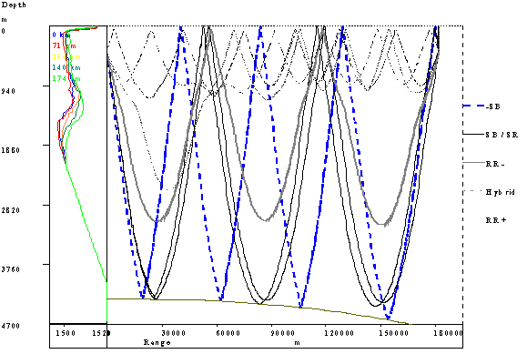
Figure 5: Ray trace in the T1T4 background environment.
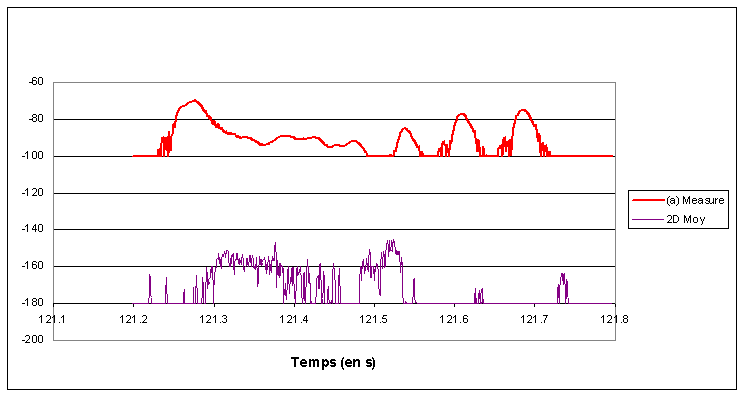
Figure 6: Averaged impulse response in the case of 50 realizations of the range dependent medium (data are recalled in the upper panel).
B. Acoustic modeling
We aim to evaluate the influence of the perturbation of the sound speed on the temporal spreading of the signal as well as on the energy repartition in the impulse response. A range dependent ray tracing model (RAYSON® , see 4.1 for details) is run for each of fifty realizations. The ray trace in the background sound speed field is presented in Figure 6. There is a significant amount of energy arriving between the first energy packet and the packet corresponding to deep refracted rays. The energy appearing between the two main packets is due to two different types of rays : deep rays reflected on the surface (SR) and deep rays refracted in the thermocline (RR-). In particular, a significant part of this energy is due to hybrid rays i.e. rays propagated in the main channel and trapped in the upper channel because of the range dependence of the environment.
The previous simulations tend to show that there indeed is energy between the two mains peaks and that the temporal spreading is consistent with what is observed on data. The range dependent model used in a statistical approach gives a good prediction of the mean impulse response that allows identification of peaks in amplitude and time of arrivals. This identification is particularly interesting for ocean tomography purposes since it increases the number of identified sound trajectories usable for inversion. The last step of this study is to check the reliability of a ray approach in a fluctuating North East Atlantic environment.
IV.
Chaotic description of the propagation
We address in this section the problem of chaotic propagation in the North East Atlantic Environment. As illustrated in
Figure 7, rays can have a chaotic behavior, which means that they are sensitive to their initial environmental conditions and to the sound speed environment. Rays with close initial conditions can have drastically different paths. These paths exponentially differ with the propagation range. It is well known that in the case of a range independent medium, ray paths are periodical [9] and that the paths are continuous with the grazing angle. Chaotic propagation can only exist in a range dependent medium. It is interesting to note that even if a “small part” of the medium is range dependent (typically several hundred of kilometers over several thousands of kilometers), the chaotic behavior of rays can drastically affect the validity of long range predictions and ray identification (
Figure 8). In particular, we can expect that predicting the propagation across the West and East Atlantic for long range tomography purposes could be difficult in reason of the presence of the Mediterranean outflow. The purpose of this work is to quantify the chaos in the Bay of Biscay and to determine the range of validity of ray approaches.
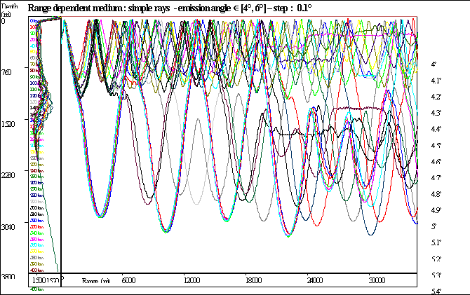
Figure 7: Illustration of the chaotic propagation in the North East Atlantic.

Figure 8: Propagation over long ranges in the case of 174 kilometers of range dependence.
A. Chaos quantification
The quantification of the chaos can be done with the Lyapunov constant [10] which enables to estimate the order of magnitude of the reliability of a ray model in the North East Atlantic. Chaotic trajectories are exponentially divergent and are characterized by a positive Lyapunov exponent:
 (2)
(2)
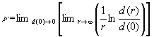
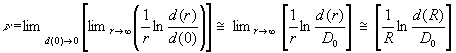
where d(r) is the separation in the phase space of two close trajectories. A chaotic trajectory (respectively a regular) is characterized by n>0 (respectively n=0). The separation d(r) is a distance which can be defined by:
![]() (3)
(3)
where z (in km) is the depth of a ray for a given range r, w is the grazing angle and z0 = 1 km. It has been shown in [11] that this method gives similar estimates of n than other methods based on the non-dimensional formulation of equation (3). It is also admitted that a deterministic prediction of chaotic rays is not possible over a range R greater than few e-folding ranges (inverse Lyapunov exponent), so when
Rn >>1 (4)
The calculus of the Lyapunov constant is introduced in the ray code RAYSON® [14] which computes the ray propagation in a range dependent environment by solving the following set of equations:
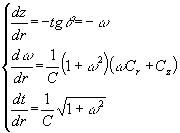 where
where
![]() (5)
(5)
This set is integrated using a Runge-Kutta of the 4th order with an adaptive step. This program is written in C++ and calculations are made in long double real offering the necessary high precision for this study. Since 1993, this program has been used and validated in many impact studies based on Monte-Carlo approach and has also been the support of the design and process of ocean acoustic experiments.
To compute the Lyapunov constant, the code traces two rays with close grazing angles. The trajectory d(r) is used to compute n, following:
 = Q(R)
(6)
= Q(R)
(6)
where D0 is the value of d(r) for a small value of r. For two rays with grazing angles q1 and q2, D0 equals:
![]() (7)
(7)
In practice, the difference of grazing angle is taken to q1 - q2 = 10-14 radians. The limit in range is taken at R=6500 km.
Another tool to estimate the chaos is to compute the spatial spectrum of the ray paths. Indeed, for a range independent medium, the ray paths are periodic. Therefore, the spatial spectrum is characterized by a single peak and several harmonics. At the opposite, in the case of a chaotic propagation, the spatial spectrum is a broadband spectrum [11]. This gives a method to estimate whether a given ray is chaotic or not.
B. Application to the propagation in the Bay of Biscay
To compute the Lyapunov constant, we build a range dependent medium over 6500 kilometers with one profile every 25 kilometers. The first five profiles are those measured between T1 and T4; the others are randomly chosen between all CTD profiles of the GASTOM experiment. Then, a random perturbation field is added in case of three different standard deviations : 0.25 m/s, 0.5 m/s and 1 m/s.
The Lyapunov constant corresponding to rays with grazing angles 5° (hereafter Ray5) and 10° (hereafter Ray10) are given in
Figure 9. Ray10 reaches faster the asymptote when the standard deviation of the perturbation is high. However, we consider here only one realization of the medium, which is not enough to make a definitive conclusion. At the opposite, Ray5 does not reach its asymptote for any value of the standard deviation presented here. If Ray10 is surely chaotic, at the opposite Ray5 has an unclear broadband spectrum and does not have clearly a non-zero asymptote. Many rays have this type of behavior, what was also noticed in [11]. When rays are chaotic but Q(R) does not reach the asymptote, we give the upper limit of the Lyapunov constant or equivalently the lower limit of predictability. Thus, Ray5 is chaotic for a range greater or equal to 1/Q(6500). However, these rays are not surely chaotic.
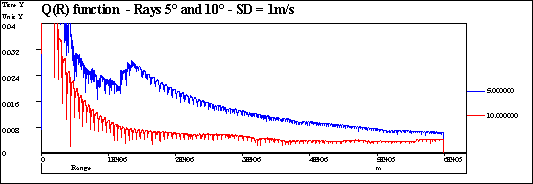
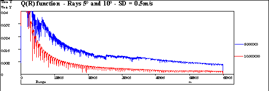
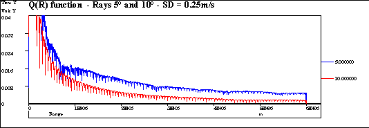
Figure 9: Lyapunov constant for rays with grazing angles 5° and 10° in the case of T1T4.
In the special case of the GASTOM experiment, the numerical evaluation is done on grazing angles in the interval [-14, 14] for three different values of standard deviation which are 0.1 m/s, 0.5 m/s and 1 m/s. The rays are classed in three types: chaotic rays when the asymptote is reached and the spectrum is broadband, uncertain chaotic when the asymptote is not reached and the spectrum is not clearly broadband and pseudo-chaotic when the spectrum is broadband but the asymptote is not reached. The limit of 1/Q(6500) is given in Figure 10. Concerning pseudo-chaotic rays, the Lyapunov exponent estimates (n = 1/180 km, nR = 0(1)) suggest that chaotic ray motion is not responsible for any apparent unpredictability in the observation. But, as they present the lower e-folding range, that means that ray predictions in the upper channel for T1T4 are the more sensitive to environmental conditions. Pseudo-chaotic rays have low grazing angles. Concerning rays with grazing angles between 5° and 15°, asymptotes are reached and n-1 extend from at least 280 to 400 km. For positive grazing angles, as shown on Figure 10, the orders of magnitude of n-1 are decreasing with the standard deviation of the perturbation field (390 km for 0.1 m/s, 371 km for 0.5 m/s and 283 km for 1 m/s).
The chaos degree has been determined in realistic case of GASTOM environment and it has been shown using few realizations that chaos is increasing with medium fluctuations. For negative grazing angles, the results are more questionable and no conclusion can be drawn. All results however have to be moderated since the simulations have not been done on a sufficient number of realizations of the perturbation medium.
C. Discussion
The results shown in this paper are consistent with what was studied in [11]. For instance, for a Munk profile, fluctuations of a 10 km wavelength and relative fluctuations of 1/1000, give a Lyapunov constant of about 1/170 km-1. In the particular case of the Bay of Biscay, this rate of fluctuation is reached for the deep maximum in the sound speed profile, as well as for the surface sound speed. The main limitation of this approach lies however, as in [11], in the ray method. Indeed, diffraction effects associated with finite frequency waves tend to reduce the sensitivity to initial conditions and environmental conditions. It can be emphasized that chaos (stricto sensu exponential sensitivity when R tends to infinity) can not exist for waves at finite frequency because they are solutions of a linear wave equation. However, numerical simulations show that such waves encompass the random features associated to chaos under the conditions for which the corresponding paths are chaotic. It is expected in [11] that, this random features, nevertheless, should be observable in the ocean for mid and large scale propagation.
Considering the case of T1T4 of GASTOM campaign we have observed and studied this random feature. A part of the energy corresponds to well-identified rays (rays trapped in the upper channel and deep refracted or bottom reflected rays). Another part of the energy is more unstable, highly fluctuating in terms of signal-to-noise ratio. This energy is put forward by averaging sequences, so by averaging several realizations of what can be considered as a random medium.
Figure 11 clearly shows
that rays with low grazing angles are highly fluctuating and that rays with
intermediate grazing angles (from -5 to -7 and from 5 to 7) are chaotic (these
rays are hybrid rays as seen in the second section of this paper). These chaotic
rays explain the distribution of the energy which appears at intermediate times
of arrival.
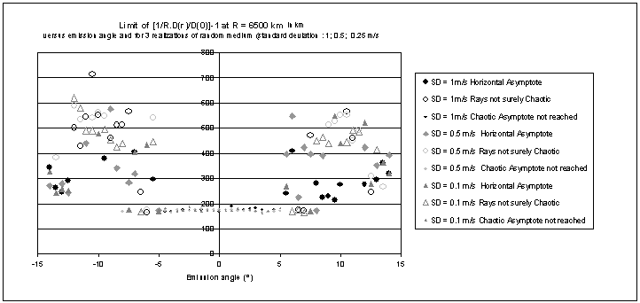
Figure 10: 1/Q(R) for the GASTOM experiment.
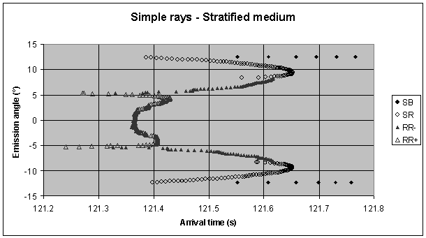
Figure 11: Grazing angles versus arrival times in the case of T1T4 environment
V.
Conclusion
The objective of this paper is to show that long range propagation can be drastically affected by mesoscale phenomena. This paper discuss the particular case of the Mediterranean outflow in the North East Atlantic. In the first part, an explanation of unpredicted energy arrivals in acoustic signals of the GASTOM experiment is given. This explanation relies upon the existence of hybrid rays which change of sound channel due to the range dependence of the medium. In the second part, an interpretation of this hybrid ray feature is given using the chaos theory. It appears that the paths of chaotic rays can not be predicted with a sufficient reliability for ranges greater or equal to a few hundred of kilometers (around 1000 km) but still remain correct in our range of application (less than 300 km). Using results and methods presented in [11], we have presented a way to determine chaos degree in our experimental case. Random features observed on real data have been linked with randomness associated with chaos. Numerical simulations, in a ray approach, has provided a better understanding of propagation in a fluctuating double sound channel.
This study will be continued by a statistical evaluation of the chaos in regards to the medium variability (in this work, only a few realizations of the medium are considered in each case). The fluctuations of arrival times and energy of the chaotic rays could be related to a measure of the background and perturbation fields. For further developments, feature models (e.g. [12]) of the Mediterranean outflow in the Bay of Biscay could be used for tomographic inversion. In addition, such models would allow to compute the second-order derivatives of the sound speed, which are required to estimate Lyapunov exponents [13]. Several data set of the GASTOM experiment (in particular with a propagation range of 300 km) could be used to illustrate this approach. Finally, the Lyapunov exponents are not perfectly adapted to measure the chaos in a double sound speed channel. Indeed, some geometrical instability can occur (for instance for rays with turning depth close to the maximum of sound speed) and this instability may not lead do a chaotic behavior, whereas the Lyapounov exponents would suggest it. In the context of double sound speed channel, it would be interesting to find a better suited criterion for chaos quantification.
ACKNOWLEDGMENT: This work was funded by the French Service Hydrographique et Océanographique de la Marine (SHOM) in the Ocean Acoustic Exploratory Development (DE95901, contract 97.87.026.00.470.29.45).
VI.
References
[1] W.H. Munk, P. Worcester and C. Wunsch, “Ocean Acoustic Tomography. Cambridge University Press, Cambridge, 1995.
[2] J.M. Darras, R. Laval and F.R. Martin-Lauzer, “Deep hydrographic fluctuations in the North East Atlantic outflow: Influence on acoustic propagation”, Ocean variability and Acoustic propagation, J. Potter & A. Warn-Varnas Eds, Kluwer, pp. 375-390, 1991
[3] Y. Stéphan, F. Evennou and F.R Martin-Lauzer, “GASTOM90: Acoustic tomography in the Bay of Biscay,” Proceedings of OCEANS96, IEEE, Fort Lauderdale, 1996.
[4] Y. Stéphan, F. Evennou, and F.R. Martin-Lauzer, “Acoustic modeling and measurements in the Bay of Biscay in a double SOFAR channel”, Full-Field Inversion Methods in Ocean and Seismo Acoustics, Diachok & Al. Eds, Kluwer, pp. 255-260, 1995.
[5] C.Noël, F. Evennou, Y. Stéphan and M.C. Pélissier, “Theoretical study of the significance and feasibility of an improvement in experimental tomography methodology through a joint assessment of arrival angles and times”, Full-Field Inversion Methods in Ocean and Seismo Acoustics, Diachok & Al. Eds, Kluwer, pp. 249-254, 1995.
[6] M. Arhan, “On the large scales dynamics of the Mediterranean outflow,” Deep-Sea Research, 34, 7, pp. 1087-1207, 1987.
[7] C. Noël, Propagation des signaux en milieux marins aléatoires, Thèse de doctorat, Université d’Aix-Marseille, 1993 (in French).
[8]
S. Flatté, R Dashen, W. Munk, K. Watson and F. Zacharisen, Sound
transmission through a fluctuating ocean,
Cambridge University Press, Cambridge, 1979.
[9]
R. Leung and H. DeFerrari, « F and L computations for real and canonical oceans ,» Journal
of Acoustical Society
of America, 67 (1), pp . 169-176, 1980.
[10] K.B. Smith, M.G. Brown and F.D. Tappert, “Ray chaos in underwater acoustics,” Journal of the Acoustical Society of America, 91(4), pp. 1939-1949, 1991a.
[11] K.B. Smith, M.G. Brown and F.D. Tappert “Acoustic ray chaos induced by mesoscale ocean structure,” Journal of the Acoustical Society of America, 91(4), pp. 1950-1959, 1991b.
[12] J. Small, L. Shackleford and G. Pavey, “Ocean feature modeling: its use on effectiveness in ocean acoustic forecasting”, Ann. Geophysicae, 15, pp. 101-112, 1997.
[13] J. Yan, “Ray chaos in underwater acoustics in view of local instability”, Journal of Acoustical Society of America, 94(5), pp. 2739-2745, 1993.
[14] Documentation about RAYSON program available on : http://pro.wanadoo.fr/semantic/
Claire NOEL received her engineer diploma from ENSMM (Mechanics and Microtechnics Engineer School) in Besançon in 1988 and her Ph.D. degree in Acoustics (sound propagation through random media) from the University of Aix-Marseille II in 1993. This work was conducted within GERDSM (DGA) in the Underwater Acoustics Department in Le Brusc.
Since 1993, she has been managing the SEMANTIC TS company that she has founded with C. Viala.; She has been working on several research projects in the domain of acoustical oceanography, acoustic propagation modeling in random ocean, ocean acoustic tomography and internal waves.
Christophe VIALA received his engineer diploma from ENSMM (Mechanics and Microtechnics Engineer School) in Besançon in 1988 and his DEA in Acousto-Opto-Electronics and Vibrations in 1989.
From 1990 to 1992, he was an engineer at GERDSM in the Submarine Radiated Noise department in Le Brusc. He co-founded the SEMANTIC TS company, in which he is the technical manager. His current research topics includes signal processing, software and measurement engineering, underwater positioning and tracking systems, ocean acoustic propagation modeling.
Yann STEPHAN was born in Lannion, France, in 1966. He received his engineering diploma in Electrical Engineering from ENSIEG in Grenoble. He received his Ph.D. degree in Computer Sciences in 1996 from CNAM in Paris. Since 1992, he has worked with the Service Hydrographique et Océanographique de la Marine (SHOM) within the Center for Military Oceanography in Brest, first as a research engineer in Ocean Acoustic Tomography, presently as the head of the Ocean Acoustics Group. His current topics include inverse methods, internal waves tomography and tactical use of the environment.